Example 1: Forward modeling of RT models (surface part)
1. Narrative (Examples of forward modeling of available RT models (surface part))
This notebook demonstrates the different available RT models (surface part) and highlights the nessesary input parameters. A short overview of the required input parameters can be found here.
Available RT models
WaterCloud
Oh92
Oh04
Dubois95
I2EM - not working right now
2. Requirements
Installation of SenSE
3. Required imports and helper function
# import packages
#-----------------
import numpy as np
import matplotlib.pyplot as plt
from sense.surface import Oh92, Oh04, Dubois95, WaterCloudSurface, I2EM
from sense.util import f2lam
from sense.dielectric import Dobson85
# Helper function
#------------------
# The RT model output is backscatter in linear units.
# For visualization in a later stage the backscatter is usually displayed in
# decibel (dB).
def db(x):
    return 10.*np.log10(x)
4. Nessesary input parameters
# Needed by all RT-models
mv = np.linspace(0.01,0.4) # soil moisture [m³/m³]
theta = np.deg2rad(40) # incidence angle [radians]

# Nessesary parameters for all except WaterCloudSurface
f  = 5.3 # Frequency [GHz]
s = 0.3/100. # surface roughness [m]

# Calculations
lam = f2lam(f)  # wavelength [m]
k = 2.*np.pi/lam # radar wave number
ks = k * s
5. Available RT models
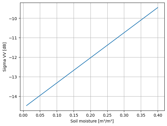
5.1 WaterCloudSurface
# Nessesary input parameters specific to Water Cloud (other parameters are
# already defined under 4. Nessesary input parameters by all RT-models)
C_vv = -14.61 # empirical factor need to calibrated for each test site
D_vv = 12.88 # empirical factor need to calibrated for each test site
C_hh = 0 # empirical factor need to calibrated for each test site
D_hh = 0 # empirical factor need to calibrated for each test site
C_hv = 0 # empirical factor need to calibrated for each test site
D_hv = 0 # empirical factor need to calibrated for each test site

# Run RT model Water Cloud (surface part)
water_cloud_surface = WaterCloudSurface(mv=mv,C_vv=C_vv,D_vv=D_vv,C_hh=C_hh,D_hh=D_hh,C_hv=C_hv,D_hv=D_hv,theta=theta)

# Plot calculated backscatter
plt.plot(mv, db(water_cloud_surface.vv))
plt.xlabel('Soil moisture [m³/m³]')
plt.ylabel('Sigma VV [dB]')
plt.grid()
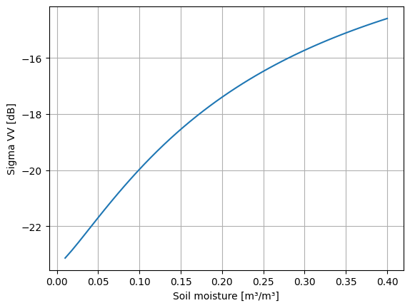
5.2 Oh92
# Oh92 needs a dielectric constant of the soil, however soil moisture values
# can be converted with the dobson model (input of clay and sand content) to
# dielectric constant values

# Nessesary input parameters specific to Oh92 (other parameters are
# already defined under 4. Nessesary input parameters by all RT-models)
sand = 0.051 # sand content of the soil
clay = 0.135 # clay content of the soil

# Convert soil moisture to dielectric constant
D = Dobson85(sand=sand, clay=clay,freq=f,mv=mv) # simplistic approach of Dobson95 model
eps = D.eps # dielectic constant values (complex; real and imaginary part)

# Run RT model Oh92
Oh92_model = Oh92(eps, ks, theta)

# Plot calculated backscatter
plt.plot(mv, db(Oh92_model.vv))
plt.xlabel('Soil moisture [m³/m³]')
plt.ylabel('Sigma VV [dB]')
plt.grid()
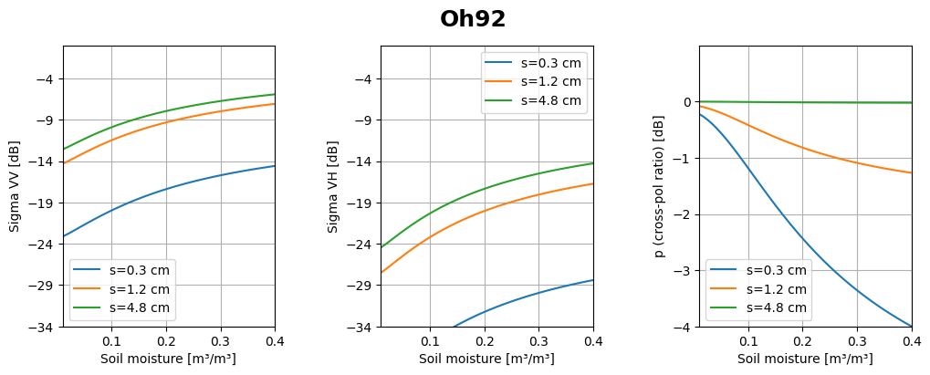
# Visualization of calculated backscatter for different surface roughness condition
#-----------------------------------------------------------------------------------
f = plt.figure(figsize=(12,4))
plt.suptitle('Oh92', fontsize=18, fontweight='bold')

ax1 = f.add_subplot(131)
ax2 = f.add_subplot(132)
ax3 = f.add_subplot(133)

s_new = 0.3/100.
ks_new = k * s_new
Oh = Oh92(eps, ks_new, theta)
ax1.plot(mv, db(Oh.vv), label=['s=0.3 cm'])
ax2.plot(mv, db(Oh.hv), label=['s=0.3 cm'])
ax3.plot(mv, db(Oh.p), label=['s=0.3 cm'])
s_new = 1.2/100.
ks_new = k * s_new
Oh = Oh92(eps, ks_new, theta)
ax1.plot(mv, db(Oh.vv), label=['s=1.2 cm'])
ax2.plot(mv, db(Oh.hv), label=['s=1.2 cm'])
ax3.plot(mv, db(Oh.p), label=['s=1.2 cm'])
s_new = 4.8/100.
ks_new = k * s_new
Oh = Oh92(eps, ks_new, theta)
ax1.plot(mv, db(Oh.vv), label=['s=4.8 cm'])
ax2.plot(mv, db(Oh.hv), label=['s=4.8 cm'])
ax3.plot(mv, db(Oh.p), label=['s=4.8 cm'])

ax1.grid()
ax1.set_xlim(0.01,0.4)
ax1.set_ylim(-34.,-0.)
ax1.set_yticks(np.arange(-34, -0, 5))
ax2.grid()
ax2.set_xlim(0.01,0.4)
ax2.set_ylim(-34.,-0.)
ax2.set_yticks(np.arange(-34, -0, 5))
ax3.grid()
ax3.set_xlim(0.01,0.4)
ax3.set_ylim(-4.,1.)
ax3.set_yticks(np.arange(-4, 1, 1))

ax1.set_xlabel('Soil moisture [m³/m³]')
ax2.set_xlabel('Soil moisture [m³/m³]')
ax3.set_xlabel('Soil moisture [m³/m³]')

ax1.set_ylabel('Sigma VV [dB]')
ax2.set_ylabel('Sigma VH [dB]')
ax3.set_ylabel('p (cross-pol ratio) [dB]')


ax1.legend()
ax2.legend()
ax3.legend()

# Adjust spacing
plt.subplots_adjust(wspace=0.5)  # Adjust the width space


plt.show()
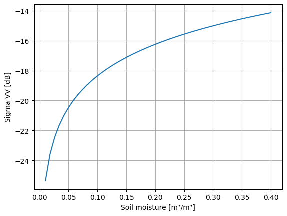
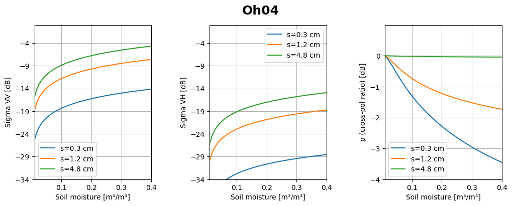
5.3 Oh04
# No additional input parameters except the ones under
# 4. Nessesary input parameters by all RT-models needed

# Run RT model Oh04
Oh04_model = Oh04(mv, ks, theta)

# Plot calculated backscatter
plt.plot(mv, db(Oh04_model.vv))
plt.xlabel('Soil moisture [m³/m³]')
plt.ylabel('Sigma VV [dB]')
plt.grid()
# Visualization of calculated backscatter for different surface roughness condition
#----------------------------------------------------------------------------------
f = plt.figure(figsize=(12,4))
plt.suptitle('Oh04', fontsize=18, fontweight='bold')

ax1 = f.add_subplot(131)
ax2 = f.add_subplot(132)
ax3 = f.add_subplot(133)

s = 0.3/100.
ks = k * s
Oh = Oh04(mv, ks, theta)
ax1.plot(mv, db(Oh.vv), label=['s=0.3 cm'])
ax2.plot(mv, db(Oh.hv), label=['s=0.3 cm'])
ax3.plot(mv, db(Oh.p), label=['s=0.3 cm'])
s = 1.2/100.
ks = k * s
Oh = Oh04(mv, ks, theta)
ax1.plot(mv, db(Oh.vv), label=['s=1.2 cm'])
ax2.plot(mv, db(Oh.hv), label=['s=1.2 cm'])
ax3.plot(mv, db(Oh.p), label=['s=1.2 cm'])
s = 4.8/100.
ks = k * s
Oh = Oh04(mv, ks, theta)
ax1.plot(mv, db(Oh.vv), label=['s=4.8 cm'])
ax2.plot(mv, db(Oh.hv), label=['s=4.8 cm'])
ax3.plot(mv, db(Oh.p), label=['s=4.8 cm'])

ax1.grid()
ax1.set_xlim(0.01,0.4)
ax1.set_ylim(-34.,-0.)
ax1.set_yticks(np.arange(-34, -0, 5))
ax2.grid()
ax2.set_xlim(0.01,0.4)
ax2.set_ylim(-34.,-0.)
ax2.set_yticks(np.arange(-34, -0, 5))
ax3.grid()
ax3.set_xlim(0.01,0.4)
ax3.set_ylim(-4.,1.)
ax3.set_yticks(np.arange(-4, 1, 1))

ax1.set_xlabel('Soil moisture [m³/m³]')
ax2.set_xlabel('Soil moisture [m³/m³]')
ax3.set_xlabel('Soil moisture [m³/m³]')

ax1.set_ylabel('Sigma VV [dB]')
ax2.set_ylabel('Sigma VH [dB]')
ax3.set_ylabel('p (cross-pol ratio) [dB]')


ax1.legend()
ax2.legend()
ax3.legend()

# Adjust spacing
plt.subplots_adjust(wspace=0.5)  # Adjust the width space

plt.show()
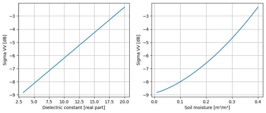
5.4 Dubois95
# Similar to 5.2 Oh92 the Dubois95 model need a dielectric constant of the soil.
# In 5.2. the conversion of soil moisture values to dielectric constant values
# wich the help of the Dobsen82 model (input of clay and sand content) was shown.
# Here we use an array dielectric constant values

import numpy as np

eps = np.array([
    3.21763781+2.37762482e-03j, 3.34171595+7.57155381e-03j,
    3.48304809+1.56444896e-02j, 3.63819338+2.65729742e-02j,
    3.80536125+4.03402087e-02j, 3.98346332+5.69330909e-02j,
    4.1717769 +7.63408799e-02j, 4.3697933 +9.85544764e-02j,
    4.57713927+1.23565989e-01j, 4.7935321 +1.51368453e-01j,
    5.01875222+1.81955635e-01j, 5.2526255 +2.15321898e-01j,
    5.49501145+2.51462093e-01j, 5.74579495+2.90371489e-01j,
    6.00488041+3.32045703e-01j, 6.27218751+3.76480658e-01j,
    6.54764798+4.23672541e-01j, 6.83120324+4.73617772e-01j,
    7.12280251+5.26312978e-01j, 7.42240141+5.81754968e-01j,
    7.72996081+6.39940719e-01j, 8.04544597+7.00867354e-01j,
    8.36882576+7.64532133e-01j, 8.70007213+8.30932438e-01j,
    9.03915962+9.00065765e-01j, 9.38606499+9.71929712e-01j,
    9.74076686+1.04652197e+00j, 10.10324549+1.12384033e+00j,
    10.47348251+1.20388265e+00j, 10.8514608 +1.28664686e+00j,
    11.23716428+1.37213099e+00j, 11.63057777+1.46033310e+00j,
    12.03168694+1.55125134e+00j, 12.44047816+1.64488390e+00j,
    12.85693843+1.74122903e+00j, 13.28105531+1.84028503e+00j,
    13.71281687+1.94205026e+00j, 14.15221162+2.04652311e+00j,
    14.59922849+2.15370203e+00j, 15.05385676+2.26358548e+00j,
    15.51608604+2.37617201e+00j, 15.98590625+2.49146015e+00j,
    16.46330756+2.60944851e+00j, 16.94828042+2.73013571e+00j,
    17.44081548+2.85352040e+00j, 17.94090362+2.97960129e+00j,
    18.4485359 +3.10837708e+00j, 18.96370357+3.23984653e+00j,
    19.48639804+3.37400840e+00j, 20.01661088+3.51086150e+00j
])

# To get just the real part as you requested:
eps_real = eps.real

# Run RT model Dubois95
Dubois95_model = Dubois95(eps=eps, ks=ks, theta=theta, lam=lam)

# Plot calculated backscatter
# As the previously defined eps values are the ones from the previously used
# Dobsen model and thus based on the previously defined soil moisture values
# both the dielectric constant and the soil moisture is plotted

f = plt.figure(figsize=(16,4))
ax1 = f.add_subplot(131)
ax2 = f.add_subplot(132)

ax1.plot(eps.real, db(Dubois95_model.vv))
ax1.set_xlabel('Dielectric constant [real part]')
ax1.set_ylabel('Sigma VV [dB]')
ax1.grid()

ax2.plot(mv, db(Dubois95_model.vv))
ax2.set_xlabel('Soil moisture [m³/m³]')
ax2.set_ylabel('Sigma VV [dB]')
ax2.grid()
5.5 I2EM
# Unfortunately using an np.array of dielectric constant/soil moisture is not
# yet supportet for I2EM. Here we show how the I2EM model changes with the
# incidence angle

# Nessesary input parameters specific to Oh92 (other parameters are
# already defined under 4. Nessesary input parameters by all RT-models)
theta_deg = np.linspace(0.,70., 71)
theta = np.deg2rad(theta_deg) # incidence angle [radians]

eps = 11.3-1.5j # dielectric constant
l = 10./100. # correlation length [m]


eps = 11.3-1.5j # dielectric constant
f = 3. # frequency [GHz]

s = 1./100. # surface roughness [m]
l = 10./100. # correlation length [m]
hh1=[]
hh2=[]
vv1=[]
vv2=[]
hv1=[]
hv2=[]
xpol = True
auto=False
for t in theta:
    print(t)
    I1 = I2EM(f, eps, s, l, t, acf_type='gauss', xpol=xpol, auto=auto)
    I2 = I2EM(f, eps, s, l, t, acf_type='exp15', xpol=xpol, auto=auto)
    print(I1.ks, I1.kl)
    hh1.append(I1.hh)
    hh2.append(I2.hh)
    vv1.append(I1.vv)
    vv2.append(I2.vv)
    if xpol:
        hv1.append(I1.hv)
        hv2.append(I2.hv)

hh1 = np.array(hh1)
hh2 = np.array(hh2)
vv1 = np.array(vv1)
vv2 = np.array(vv2)
hv1 = np.array(hv1)
hv2 = np.array(hv2)
0.0
---------------------------------------------------------------------------
UnboundLocalError                         Traceback (most recent call last)
Cell In[11], line 11
      9 for t in theta:
     10     print(t)
---> 11     I1 = I2EM(f, eps, s, l, t, acf_type='gauss', xpol=xpol, auto=auto)
     12     I2 = I2EM(f, eps, s, l, t, acf_type='exp15', xpol=xpol, auto=auto)
     13     print(I1.ks, I1.kl)

File ~/checkouts/readthedocs.org/user_builds/sense-community-sar-scattering-model/envs/dev/lib/python3.10/site-packages/sense/surface/i2em.py:92, in I2EM.__init__(self, f, eps, sig, l, theta, **kwargs)
     88 self.init_model()
     89 # pdb.set_trace()
     90
     91 # calculate the actual backscattering coefficients
---> 92 self._calc_sigma_backscatter()

File ~/checkouts/readthedocs.org/user_builds/sense-community-sar-scattering-model/envs/dev/lib/python3.10/site-packages/sense/surface/i2em.py:191, in I2EM._calc_sigma_backscatter(self)
    189 self._init_hlp()
    190 self.init_model()
--> 191 self.vv, self.hh = self._i2em_bistatic()
    192 if self.xpol:
    193     self.hv = self._i2em_cross()

File ~/checkouts/readthedocs.org/user_builds/sense-community-sar-scattering-model/envs/dev/lib/python3.10/site-packages/sense/surface/i2em.py:207, in I2EM._i2em_bistatic(self)
    204 self.fac = [math.factorial(x) for x in idx]
    206 self.wn, self.rss = self.calc_roughness_spectrum(acf_type=self.acf_type)
--> 207 Ivv, Ihh = self._calc_Ipp()
    208 Ivv_abs = np.abs(Ivv)
    209 Ihh_abs = np.abs(Ihh)

File ~/checkouts/readthedocs.org/user_builds/sense-community-sar-scattering-model/envs/dev/lib/python3.10/site-packages/sense/surface/i2em.py:410, in I2EM._calc_Ipp(self)
    407 Rhi = R.rho_h
    409 Fvvupi, Fhhupi = self.Fppupdn( 1,1,Rvi,Rhi)
--> 410 Fvvups, Fhhups = self.Fppupdn( 1,2,Rvi,Rhi)
    411 Fvvdni, Fhhdni = self.Fppupdn(-1,1,Rvi,Rhi)
    412 Fvvdns, Fhhdns = self.Fppupdn(-1,2,Rvi,Rhi)

File ~/checkouts/readthedocs.org/user_builds/sense-community-sar-scattering-model/envs/dev/lib/python3.10/site-packages/sense/surface/i2em.py:592, in I2EM.Fppupdn(self, u_d, i_s, Rvi, Rhi)
    589 q = self._kz
    590 qt = self.k * np.sqrt(self.eps - self._s**2.)
--> 592 vv =  (1.+Rvi) *( -(1-Rvi) *c11 /q + (1.+Rvi)       *c12 / qt)
    593 vv += (1.-Rvi) *(  (1-Rvi) *c21 /q - (1.+Rvi)       *c22 / qt)
    594 vv += (1.+Rvi) *(  (1-Rvi) *c31 /q - (1.+Rvi)       *c32 /self.eps /qt)

UnboundLocalError: local variable 'c11' referenced before assignment
f = plt.figure()
ax = f.add_subplot(111)

# ax.plot(theta_deg, db(hh2), color='red', label='hh')
ax.plot(theta_deg, db(hh1), color='blue', label='hh')

# ax.plot(theta_deg, db(vv2), color='red', label='vv', linestyle='--')
ax.plot(theta_deg, db(vv1), color='blue', label='vv', linestyle='--')

# ax.plot(theta_deg, db(hv2), color='red', label='hv', linestyle='-.')
ax.plot(theta_deg, db(hv1), color='blue', label='hv', linestyle='-.')

ax.grid()
ax.set_xlim(0.,70.)
ax.set_ylim(-100.,15.)
ax.set_yticks(np.arange(-90, 20, 10))
plt.ylabel('Backscatter [dB]')
plt.xlabel('Incidence angle [°]')
plt.legend()
plt.show()